Logistic Equation Variations
The colors represent Poincare Recurrance times for omega along the
horizontal axis, and lambda along the vertical axis. Remember -- click
on the small image to get a big view.

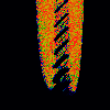
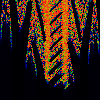
 From left to right:
- Sin
- x[n+1] = lambda * sin (pi * (x[n]-omega)) mod 1
- Gauss
- x[n+1] = lambda * exp (pi * (x[n]-omega)^2) mod 1
- Sinc
- x[n+1] = lambda * sinc (pi * (x[n]-omega)) mod 1
where sinc(y) = sin(y) / y
- Expand
- Let y = x[n] - 1/ (omega-0.5) and z = x[n] + 1/ (omega-0.5)
Then x[n+1] = lambda * y * z
Expansions and Distortions
All of the below represent the standard logistic equation; they differ
merely in the coordinate mapping. That is, they are really the same
picture, just distorted.

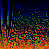
 From left to right:
- Squash
- y = x[n] - omega, z = x[n] + omega,
x[n+1] = lambda * y * (1-z) mod 1
- Flip
- y = x[n] - omega, z = x[n] + omega,
x[n+1] = (1/lambda) * y * (1-z) mod 1
- Sku
- y = x[n] - (omega-0.5)/lambda + 0.5
z = x[n] + (omega-0.5)/lambda + 0.5
x[n+1] = y * (1-z) mod 1


 From left to right:
- Squirt
- y = x[n] - (omega-0.5)/sqrt(lambda) + 0.5
z = x[n] + (omega-0.5)/sqrt(lambda) + 0.5
x[n+1] = y * (1-z) mod 1
- Stret
- y = x[n] - sqrt (omega / lambda) + 0.5
z = x[n] + sqrt (omega / lambda) + 0.5
x[n+1] = y * (1-z) mod 1
- Tch
- Same equation as Stret, different domain.
Copyright © 1996 Linas Vepstas

Logistic Equation Variations
by Linas Vepstas is licensed under a
Creative Commons
Attribution-ShareAlike 4.0 International License.


 From left to right:


 From left to right:


 From left to right:
